
Skip Nav Destination
Close Modal


![Ultrastructural organization of microtubules in the outer segment of haltere campaniform receptors. (A) Cartoon schematic of the sensory neuron in haltere receptors. BB, basal body. (B) The localizations of NompC-GFP (MO), Mks1-GFP (transition zone [TZ]), and GFP-Cnn1 (BB) in haltere receptors (top view). Upper: nompC-gfp-KI. Middle: Mks1-gfp. Lower: uas-gfp-cnn1/+; +/+; dcx-emap-gal4/+. Scale bar, 5 µm. (C–F) Cross-sectional views of the MO (C), neck (D), TB (E), and cilium (F). (G) Lateral view of the cilium. Black arrowhead, a doublet. (H) Lateral view of the mother centriole (MC), daughter centriole (DC), and cilium. Scale bars (C–H), 250 nm. C–H are ET slice images. (I) Reconstructed model of microtubules in the outer segment. Each microtubule was shown as a rod. White, microtubule in the outer segment. Red (tubule-A) and green (tubule-B), doublet. Yellow, microtubule in the inner segment. Scale bar, 1 µm. Also see Video 1.](https://cdn.rupress.org/rup/content_public/journal/jcb/220/1/10.1083_jcb.202004184/3/s_jcb_202004184_fig1.png?Expires=2147483647&Signature=BIBijU88Nf0P2p2eo5glEsjjvJuazph0kxHr1NG4PnW9wzFyLfPXIllAniaPrN~aRrXufL-t0I6OKTX1HgiwSyOKoZUpqAKhXo-o183QJYikB9OxUuP5A1noDC5W0ohXIgfeDEvTMR4dFlD7uOtLFi7hrjHIXTU7~fe-4PZ8k-4sdmZkbQEd8bLoUN0V1iLNAqGlPu3P3LWqO4cdFiC61TQJ2RYZPJYpUOgDoLWi-AbUs6KW~E~dM4GbfxVA28yijzuHvODdo4Gml~LxGXuvJ0JfcuDkVW3vdYLAHcOzYMP4U2-sT19ui172iYDwNpJXg-roqsmAIu4vFiSqU5bnEQ__&Key-Pair-Id=APKAIE5G5CRDK6RD3PGA)
![Ultrastructural organization of microtubules in the outer segment of leg campaniform receptors. (A) Cartoon schematic of the sensory neuron in leg receptors. (B) The localizations of NompC-GFP (MO), Mks1-GFP (transition zone [TZ]), and GFP-Cnn1 (basal body [BB]) in leg receptors (lateral view). Upper: nompC-gfp-KI; dcx-emap-gal4, uas-cd4-tdTom/+. Middle: +/Mks1-gfp; +/dcx-emap-gal4, uas-cd4-tdTom. Lower: uas-gfp-cnn1/+; +/+; dcx-emap-gal4, uas-cd4-tdTom/+. Scale bar, 5 µm. (C) Lateral view (ET slice image) of the outer segment. Red arrowhead, a TB microtubule. (D) Reconstructed model of microtubules in the outer segment. Blue, MO microtubule. White, TB microtubule. Red (tubule-A) + green (tubule-B), doublet. (E) Spatial distribution of microtubule ends in the outer segment. Every spot represented one end. Green, distal end. Red, proximal end. The yellow line (yellow arrowhead) indicates the distal tip. Scale bars (C–E), 500 nm. (F) The distribution of the distance between each microtubule end to the distal tip (representative of data from five cells). Red, proximal end. Green, distal end. The pie chart shows the percentage of MO microtubules that had the proximal end (p-end) in the TB. MT, microtubule; mem, membrane.](https://cdn.rupress.org/rup/content_public/journal/jcb/220/1/10.1083_jcb.202004184/3/s_jcb_202004184_fig2.png?Expires=2147483647&Signature=oO7L~RFFeojJ~tM8pSHxVWH1mVh~P7Rx1XSPNi8YiAig6Z6l6ZjVtOI~GsS2mMqH0~1iC4xRj5SU243VBED7W9gNkf7DQpxywz6CjiBzZaZekxYBBsAhGBTzOEm5eQ3TluEwQBHFBWoVXOXqiCP98j-eChG8oUIBoxdJVzRDU2dvtSfNiWPEaXahJUxalSKqp-cFkMm108fhc0WzbQwJsELHKGEaG6CA1oN4mqTz3Z30rrXVB2d07jQZl-DeZNA8R~8k-J5IJFyNixx1e2IExxJ5h9~-PrZBZYdTFbSo-TWJwmPN1~AD-FXwEf2-h15JacqVfux9gYs1vU14YkIiQQ__&Key-Pair-Id=APKAIE5G5CRDK6RD3PGA)


1-20 of 116
Follow your search
Access your saved searches in your account
Would you like to receive an alert when new items match your search?
1
Journal Articles
Journal:
Journal of Cell Biology
J Cell Biol (2020) 220 (2): e202010039.
Published: 16 December 2020
in 3D FIB-SEM reconstruction of microtubule–organelle interaction in whole primary mouse β cells
> Journal of Cell Biology
Published: 16 December 2020
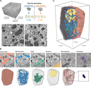
Figure 1. FIB-SEM volumes of pancreatic β cells and 3D segmentation of microtubules and organelles. (A) Full FIB-SEM volume of a pancreatic islet (left), one of which was acquired for low- and high-glucose conditions containing three (low) and More about this image found in FIB-SEM volumes of pancreatic β cells and 3D segmentation of microtubules a...
in 3D FIB-SEM reconstruction of microtubule–organelle interaction in whole primary mouse β cells
> Journal of Cell Biology
Published: 16 December 2020
Figure S1. Raw FIB-SEM data and workflow for sample preparation, imaging, segmentation, and data integration within BetaSeg Viewer. (A) Snapshots of samples prepared according to the old and new freeze substitution protocol. Arrowhead, More about this image found in Raw FIB-SEM data and workflow for sample preparation, imaging, segmentation...
in 3D FIB-SEM reconstruction of microtubule–organelle interaction in whole primary mouse β cells
> Journal of Cell Biology
Published: 16 December 2020
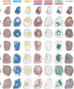
Figure S2. 3D renderings of all β cells and organelles/organelle subtypes analyzed in this study. Color-coded are microtubule-associated and –not associated SGs, mitochondria, nuclei, microtubules, centrioles, centrosomal microtubules, Golgi More about this image found in 3D renderings of all β cells and organelles/organelle subtypes analyzed in ...
in 3D FIB-SEM reconstruction of microtubule–organelle interaction in whole primary mouse β cells
> Journal of Cell Biology
Published: 16 December 2020
Figure 2. Microtubule network properties and distance distributions. (A) Fully reconstructed microtubule network of one β cell with microtubules in red, centrioles in purple, Golgi apparatus in green, and plasma membrane (PM) in gray More about this image found in Microtubule network properties and distance distributions. (A) Fully recon...
in 3D FIB-SEM reconstruction of microtubule–organelle interaction in whole primary mouse β cells
> Journal of Cell Biology
Published: 16 December 2020
Figure S3. Microtubule and SG analysis for all cells . (A) Distance of microtubule ends to the nucleus. (B) Distance of microtubule ends to Golgi (bin 20 nm). (C) Distance of microtubule ends to Golgi (bin 200 nm). (D) Distance of More about this image found in Microtubule and SG analysis for all cells . (A) Distance of microtubule e...
in 3D FIB-SEM reconstruction of microtubule–organelle interaction in whole primary mouse β cells
> Journal of Cell Biology
Published: 16 December 2020
Figure 3. Insulin SG properties and distance distributions. (A) Volume fraction (percentage) of segmented organelles for all analyzed cells. (B) 3D rendering of one β cell with plasma membrane (transparent gray), insulin SGs (orange), Golgi More about this image found in Insulin SG properties and distance distributions. (A) Volume fraction (per...
in 3D FIB-SEM reconstruction of microtubule–organelle interaction in whole primary mouse β cells
> Journal of Cell Biology
Published: 16 December 2020
Figure 4. Spatial association between microtubules and insulin SGs. (A) 3D rendering of a cell with plasma membrane (transparent gray), microtubules (red), and insulin SGs (orange). Inset shows a magnified region. Scale: cube with a side length More about this image found in Spatial association between microtubules and insulin SGs. (A) 3D rendering...
Journal Articles
In Special Collection:
Structural Biology 2021
Journal:
Journal of Cell Biology
J Cell Biol (2020) 220 (1): e202004184.
Published: 02 December 2020
Published: 02 December 2020
Figure 1. Ultrastructural organization of microtubules in the outer segment of haltere campaniform receptors. (A) Cartoon schematic of the sensory neuron in haltere receptors. BB, basal body. (B) The localizations of NompC-GFP (MO), Mks1-GFP More about this image found in Ultrastructural organization of microtubules in the outer segment of halter...
Published: 02 December 2020
Figure 2. Ultrastructural organization of microtubules in the outer segment of leg campaniform receptors. (A) Cartoon schematic of the sensory neuron in leg receptors. (B) The localizations of NompC-GFP (MO), Mks1-GFP (transition zone [TZ]), More about this image found in Ultrastructural organization of microtubules in the outer segment of leg ca...
Published: 02 December 2020
Figure S1. KI strains and live-cell imaging of leg campaniform mechanoreceptors. (A) Cartoon schematic for the NompC-GFP KI strain (nompC-gfp-KI). The insertion site of GFP was indicated. (B) Localization of NompC-GFP (nompC-gfp-KI) in fly More about this image found in KI strains and live-cell imaging of leg campaniform mechanoreceptors. (A) ...
Published: 02 December 2020
1

