
1-20 of 119915
Follow your search
Access your saved searches in your account
Would you like to receive an alert when new items match your search?
Journal Articles
Journal Articles
Published: 18 June 2026
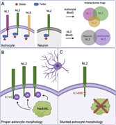
Figure 1. NLs are functionally diverse, and astrocytic NL2 is ubiquitinated by Nedd4l for proper astrocyte morphogenesis. (A) The authors used in vivo BioID to identify the interactomes for astrocyte NL1–3 and neuronal NL2. (B) In wild-type More about this image found in NLs are functionally diverse, and astrocytic NL2 is ubiquitinated by Nedd4l...
Journal Articles
Journal:
Journal of Cell Biology
J Cell Biol (2026) 225 (8): e202509200.
Published: 12 June 2026
Includes: Supplementary data
Journal Articles
Journal Articles
in Redox-dependent S-glutathionylation of Aurora-A kinase by Gstp promotes postsynaptic maturation
> Journal of Cell Biology
Published: 12 June 2026
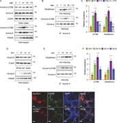
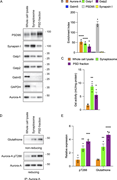
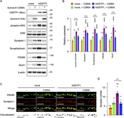
Figure 1. Aurora-A is specifically activated and glutathionylated at the PSD during the peak window of synaptogenesis. (A–C) Developmental profile of Aurora-A modification in the murine brain. (A and B) PSD fractions were prepared from murine More about this image found in Aurora-A is specifically activated and glutathionylated at the PSD during t...
in Redox-dependent S-glutathionylation of Aurora-A kinase by Gstp promotes postsynaptic maturation
> Journal of Cell Biology
Published: 12 June 2026
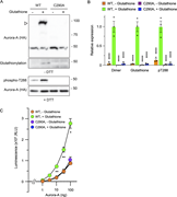
Figure 2. C290 glutathionylation promotes Aurora-A dimerization and autophosphorylation. (A) Cortical neurons from murine E14 embryos were cultured for the indicated number of DIV following adenoviral infection. Representative immunoblots show More about this image found in C290 glutathionylation promotes Aurora-A dimerization and autophosphorylati...
in Redox-dependent S-glutathionylation of Aurora-A kinase by Gstp promotes postsynaptic maturation
> Journal of Cell Biology
Published: 12 June 2026
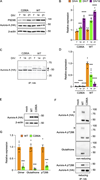
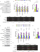
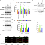
Figure 3. Gstp-mediated glutathionylation of Aurora-A is required for synaptogenesis. (A) RT-qPCR screening of 18 cytoplasmic Gst isoforms in cultured cortical neurons. Among the isoforms tested, Gstp1 and Gstp2 exhibited the highest More about this image found in Gstp-mediated glutathionylation of Aurora-A is required for synaptogenesis....
in Redox-dependent S-glutathionylation of Aurora-A kinase by Gstp promotes postsynaptic maturation
> Journal of Cell Biology
Published: 12 June 2026
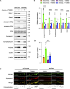
Figure 4. Co-enrichment of Aurora-A and Gstp at the PSD in the mouse brain . (A) Representative immunoblots of biochemical fractions prepared from P14 murine brain lysates. Whole-brain lysate, synaptosome, and detergent-extracted PSD fractions More about this image found in Co-enrichment of Aurora-A and Gstp at the PSD in the mouse brain . (A) Re...
in Redox-dependent S-glutathionylation of Aurora-A kinase by Gstp promotes postsynaptic maturation
> Journal of Cell Biology
Published: 12 June 2026
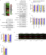
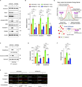
Figure 5. C290 glutathionylation potentiates Aurora-A kinase activity. (A–C) In vitro glutathionylation promotes T288 autophosphorylation and enhances the kinase activity of WT Aurora-A, but not of the C290A mutant. Purified recombinant More about this image found in C290 glutathionylation potentiates Aurora-A kinase activity. (A–C) In vitr...
in Redox-dependent S-glutathionylation of Aurora-A kinase by Gstp promotes postsynaptic maturation
> Journal of Cell Biology
Published: 12 June 2026
Figure 6. Redox-mediated potentiation of Aurora-A at C290 is required for Aurora-A to reach the full functional threshold for synapse assembly. Cortical neurons from murine E14 embryos were cultured and infected with adenovirus vectors More about this image found in Redox-mediated potentiation of Aurora-A at C290 is required for Aurora-A to...
in Redox-dependent S-glutathionylation of Aurora-A kinase by Gstp promotes postsynaptic maturation
> Journal of Cell Biology
Published: 12 June 2026
Figure 7. Constitutively active Aurora-A rescues synaptogenesis defects caused by Gstp knockdown. Aurora-A T288D restores synaptic marker expression in Gstp-deficient neurons. (A) Representative immunoblots of the indicated proteins. Cortical More about this image found in Constitutively active Aurora-A rescues synaptogenesis defects caused by ...
in Redox-dependent S-glutathionylation of Aurora-A kinase by Gstp promotes postsynaptic maturation
> Journal of Cell Biology
Published: 12 June 2026
Figure 8. Human GSTP1 enhances synaptogenesis via Aurora-A activation. Overexpression of hGSTP1 promotes synaptic marker expression. (A) Representative immunoblots of the indicated proteins. Cortical neurons were co-electroporated with More about this image found in Human GSTP1 enhances synaptogenesis via Aurora-A activatio...
in Redox-dependent S-glutathionylation of Aurora-A kinase by Gstp promotes postsynaptic maturation
> Journal of Cell Biology
Published: 12 June 2026
Figure 9. Redox-dependent regulation of Aurora-A glutathionylation and synaptogenesis. Impact of redox reagents on synaptic marker expression. (A) Representative immunoblots for the indicated proteins, confirming the effects of the oxidant H2O More about this image found in Redox-dependent regulation of Aurora-A glutathionylation and synaptogenesis...
in Redox-dependent S-glutathionylation of Aurora-A kinase by Gstp promotes postsynaptic maturation
> Journal of Cell Biology
Published: 12 June 2026
Figure 10. Gstp acts as a kinetic facilitator to ensure efficient redox-dependent Aurora-A activation. ( A and B) H2O2 treatment partially restores synaptic marker expression in Gstp-deficient neurons. (A) Representative immunoblots for the More about this image found in Gstp acts as a kinetic facilitator to ensure efficient redox-dependent Auro...
in Met-Vision reveals coexisting energetic states in tissue macrophages redistributed by inflammation
> Journal of Cell Biology
Published: 12 June 2026
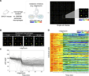
Figure 1. Met-Vision, an imaging-based automated pipeline to profile energy metabolism at the single-cell level. (A) Principle for Met-Vision analyses. Macrophages isolated from SPICY mice expressing the PercevalHR fluorescent reporter for More about this image found in Met-Vision, an imaging-based automated pipeline to profile energy metabolis...
in Met-Vision reveals coexisting energetic states in tissue macrophages redistributed by inflammation
> Journal of Cell Biology
Published: 12 June 2026
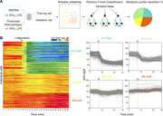
Figure 2. Met-Vision identifies and classifies distinct energy metabolism profiles in macrophages. (A) Scheme illustrating the main steps to establish a classifier for macrophage energy metabolic profiles. The dataset (n = 879 macrophages) More about this image found in Met-Vision identifies and classifies distinct energy metabolism profiles in...
in Met-Vision reveals coexisting energetic states in tissue macrophages redistributed by inflammation
> Journal of Cell Biology
Published: 12 June 2026
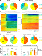
Figure 3. Distinct macrophage metabolic profiles coexist at steady state and are reconfigured upon inflammation. (A and B) Distribution of the four metabolic profiles (Ox-high, Ox-med, Ox-low, and Ox-null) in (A) BMDMs treated or not with More about this image found in Distinct macrophage metabolic profiles coexist at steady state and are reco...

