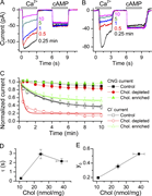
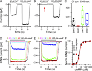
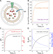
Figure 1. TMEM16B, but not CNG, current run-down is cholesterol dependent. (A and B) TMEM16B and CNGA2 current traces for control (A) and cholesterol-depleted (MβCD-treated) (B) patches at a holding potential of −40 mV. (C and D) Current More about this image found in TMEM16B, but not CNG, current run-down is cholesterol dependent. (A and B) ...

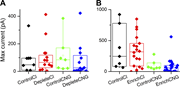
Figure 2. Comparison of peak currents measured from the first recording immediately following patch excision. (A and B) Neither (A) cholesterol depletion nor (B) cholesterol enrichment changed the average currents of both TMEM16B and CNGA2 More about this image found in Comparison of peak currents measured from the first recording immediately f...

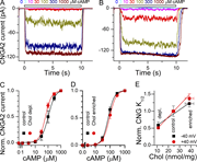
Figure 3. CNGA2 channel sensitivity to cAMP is cholesterol dependent. (A and B) CNGA2 current traces for control (A) and cholesterol-depleted (MβCD-treated) (B) patches elicited by increasing concentrations of cAMP, applied for 10 s. Holding More about this image found in CNGA2 channel sensitivity to cAMP is cholesterol dependent. (A and B) CNGA...

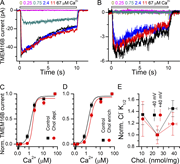
Figure 4. TMEM16B channel sensitivity to Ca²⁺ is cholesterol dependent. (A and B) TMEM16B current traces for control (A) and cholesterol-depleted (B) patches elicited by increasing concentrations of Ca²⁺, applied for 10 s. Holding potential was More about this image found in TMEM16B channel sensitivity to Ca²⁺ is cholesterol dependent. (...

Figure 5. Cholesterol depletion leads to a complete loss of the native Cl ⁻ current in membrane patches excised from dendritic knobs of mouse ORNs. Excised patches were exposed for 3 s to saturating concentrations of Ca²⁺ and cAMP to activate More about this image found in Cholesterol depletion leads to a complete loss of the native Cl ⁻ ...

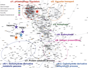
Figure 1. Selection of representative ion transporters from all known human lysosomal proteins for model construction. Proteins were annotated under the Gene Ontology Cellular Component term GO:0005764 lysosome, H. sapiens. Stars denote proteins More about this image found in Selection of representative ion transporters from all known human lysosomal...

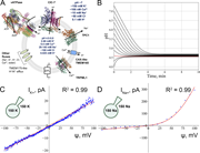
Figure 2. Representation of the model. (A) Schematic illustration of ion transporters and passive ions/water fluxes implemented in the model. Protein positions within the membrane were predicted using the Assignment aNd VIsualization of the More about this image found in Representation of the model. (A) Schematic illustration of ion transporter...

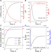
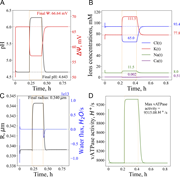
Figure 3. Modeling of lysosome maturation. (A) vATPases number increases while Na⁺/K⁺-ATPases number decreases during lysosome maturation. (B) Shift of pH and membrane potential of endosomes toward near-lysosomal levels. (C) Kinetics of ion More about this image found in Modeling of lysosome maturation. (A) vATPases number increases while Na...

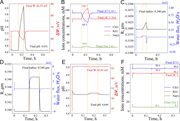
Figure 4. Consequences of transient LMP modeled as a 100-fold increase in membrane permeabilities. (A) Increase in pH and decrease in potential. (B) Adjustments of K⁺, Na⁺, and Cl⁻ ions concentrations. Colored numbers indicate concentrations More about this image found in Consequences of transient LMP modeled as a 100-fold increase in membrane pe...

Figure 5. Short-term stress simulations. vATPase knockout as a model of adaptation to the metabolic shift from catabolism to anabolism. (A) Increase in pH and decrease in membrane potential. (B) Cation influx and Cl⁻ efflux. (C) Modest More about this image found in Short-term stress simulations. vATPase knockout as a model of adaptation t...

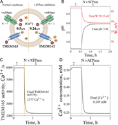
Figure 6. Lysosomal calcium depletion following vATPase inhibition. (A) In silico experiment setup. Schematic illustration of the lysosomal response to vATPase inhibition, showing resulting changes in TMEM165 activity and [Ca²⁺]. (B) Increase More about this image found in Lysosomal calcium depletion following vATPase inhibition. (A) In si...

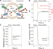
Figure 7. Lysosomal calcium concentration decrease following deacidification via additional proton efflux. (A) In silico experiment setup. Schematic illustration of the lysosomal response to direct proton efflux. (B) Changes in pH and More about this image found in Lysosomal calcium concentration decrease following deacidification via addi...

Figure 8. Accumulation of weakly basic, proton sponge-like CADs. (A) Schematic illustration of increased osmotic pressure and lysosomal swelling due to Sps accumulation. The diagram depicts the relationship between proton binding to Sps and the More about this image found in Accumulation of weakly basic, proton sponge-like CADs. (A) Schematic illus...

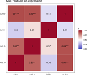
Figure 1. Correlation of SUR and Kir in mouse AT muscle. Data from Staunton et al. (2022) analysis here Barrett-Jolley (2026) . Includes healthy young and old mice; 10 RNA sequence samples in total. Note that this figure does not indicate More about this image found in Correlation of SUR and Kir in mouse AT muscle. Data from Staunton et al. ...

(Clockwise from top left) Valeriy Lukyanenko, Joaquin Muriel, Robert Bloch, and Noah Weisleder. Four headshots show Valeriy Lukyanenko at top left, Joaquin Muriel at top right, Robert Bloch at bottom right, and Noah Weisleder at bottom left. More about this image found in (Clockwise from top left) Valeriy Lukyanenko, Joaquin Muriel, Robert Bloch,...

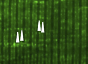
Lukyanenko et al. show that a chimeric protein containing two PKCαC2 domains and the C2A domain of dysferlin localizes to triad junctions (white arrowheads) in dysferlin-deficient myofibers. The C2A domain supports both normal Ca²⁺ signaling and More about this image found in Lukyanenko et al. show that a chimeric protein containing two PKCαC2 domain...